Examples

Holography

The example here describes the process followed by the function dichroism() in the examples.py file. More specifically, Fourier transform holography is used to recover the out-of-plane (\(z\) component) magnetization in the sample by harnessing x-ray magnetic circular dichroism (XMCD).

Initializations

The example below uses the labyrinthine domain pattern supplied with the package:

First, the experimental setup and sample is specified using the Sample, Beam and Geometry classes. The sample length describes the real-space size of the numpy array mag_config (end-to-end dimension).

Subsequently, two beam’s are described: a circular left polarized beam, with stokes parameters [1, 0, 0, 1] and a circular right polarized beam, with stokes parameters [1, 0, 0, -1]. The wavelength and full-width at half maximum (provided in meters) are also necessary for the experiment.

Then, a geometry class is created that contains information such as the distance between the sample and detector and the angle of incidence of the beam.

# create the sample
sample = scatter.Sample(sample_length, scattering_factors, mag_config)

# create a circular left and circular right polarized beam, sensitive to the z component
beam_cp = scatter.Beam(scatter.en2wave(energy), [fwhm, fwhm], pol_dict['CL'])
beam_cl = scatter.Beam(scatter.en2wave(energy), [fwhm, fwhm], pol_dict['CR'])

# describe the geometry
geometry = scatter.Geometry(angle, detector_distance)

Scattering

The scattering pattern is calculated as soon as the Scatter object is created. The Scatter class takes the experimental parameters defined above, namely the beam, sample and geometry, in order to calculate the expected scattering pattern:

s_cp = scatter.Scatter(beam_cp, sample, geometry)
s_cl = scatter.Scatter(beam_cl, sample, geometry)

Plotting Scattering Patterns

To zoom in on a specific section of the scattering pattern to re-calculate it with finer details, the function plot.intensity_interactive(Scatter) can be used.

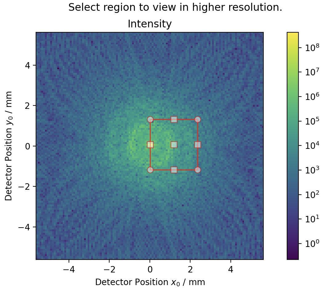
# bring up interactive intensity plot to select region of interest
returned_roi = plot.intensity_interactive(s_cp, log=True)

# the selected region is provided to the scattering classes and the calculation is performed again
s_cl.roi = returned_roi
s_cp.roi = returned_roi

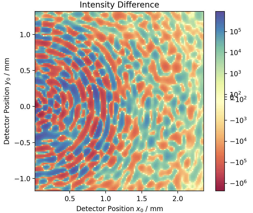
When a parameter of the scattering class is updated, the scattering is re-evaluated to match the new parameter. Here, by updating the roi parameter, the scattering patterns are updated. Then, the difference between the scattering patterns obtained using circular left and circular right polarizations can be plotted using:

plot.difference(s_cl, s_cp, log=True)
plt.show()

This gives the following figure, where the scattering pattern within the region of interest is plotted. This reveals a difference in the scattered intensities between the two polarizations, concentric rings due to the circular object, and a higher intensity ring around \(1.75~\text{mm}\) due to the size of the domains.

Preparing Sample for Holography

For holography to work, a reference hole is necessary. This can be introduced by calling the function

holography_reference(sample, reference_hole_size, 'xy')

This adds the smallest possible padding and reference hole to allow a full reconstruction. In this example, holes are added in both \(x\) and \(y\) directions. Again, by changing the sample class automatically updates the scattering pattern.

Viewing Holography Reconstruction

The scattering pattern can be inverted using the invert_holography(...) function in the holography.py file. This is automatically done by calling the plotting function:

plot.holography(s_cp, s_cl, log=True, recons_only=False)  # entire pattern
plot.holography(s_cl, s_cp)  # only sample reconstruction
plt.show()

The first call plots the entire holographic reconstruction (left panel), which contains a large central part caused by the auto-correlation of the structure with itself. On the position of the reference holes, it is now possible to see the reconstruction of the \(m_z\) component of the magnetization. This is because the reference hole has been convolved with the magnetic structure, and since the reference hole is similar to the \(\delta\) function, the structure is recovered. Complex conjugate reconstructions appear at mirror-symmetric locations. The second call in the example code only focuses on the reconstruction (right panel)

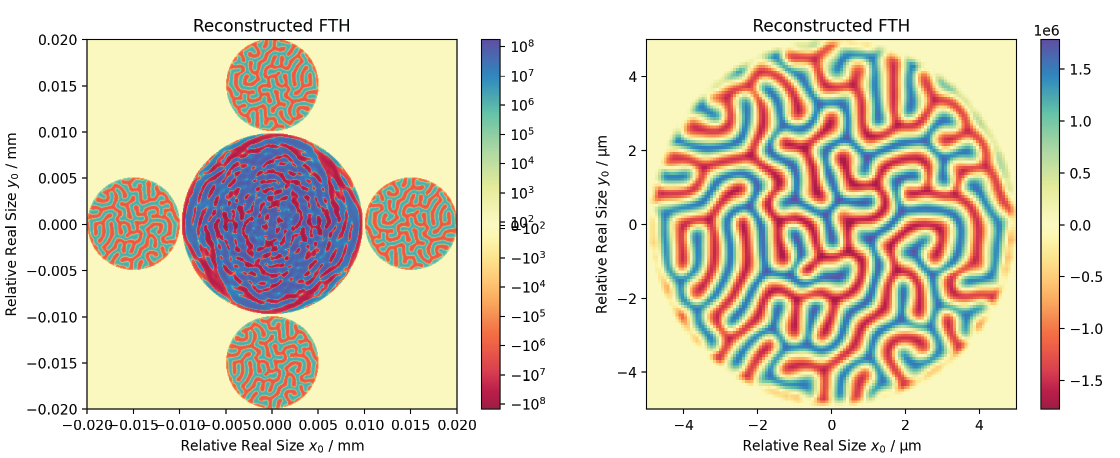
Comparing the \(m_z\) component in the initial structure (from the first figure) with the final reconstruction, it can be seen that the magnetization was correctly recovered.

Full Code

The full code from the examples.py file can be seen here:

View Code

import numpy as np
from magneticScattering import scatter, plot
import matplotlib.pyplot as plt
from magneticScattering.holography import holography_reference
from importlib import resources
import magneticScattering.data
import gzip

pol_dict = {'LH': [1, 1, 0, 0], 'LV': [1, -1, 0, 0],
            'CL': [1, 0, 0, 1], 'CR': [1, 0, 0, -1]}


def dichroism():
    """Simulated the circular magnetic dichroism from a labyrinthine pattern.

    See :ref:`example` for a more detailed description."""
    energy = 706  # energy of the beam in eV
    fwhm = 20e-6  # full width at half maximum of the beam in meters
    angle = 0  # angle of incidence
    detector_distance = 50e-2  # sample-detector distance
    sample_length = 10e-6  # sample size
    scattering_factors = [1j + 1, 1j + 1, 1 + 1j]  # scattering factors
    reference_hole_size = 3 # size of reference hole in pixels

    # load magnetic configuration
    inp_file = resources.files(magneticScattering.data) / 'labyrinthine.npy.gz'

    # Open it using gzip
    with inp_file.open("rb") as raw_f:
        with gzip.GzipFile(fileobj=raw_f, mode="rb") as gz_f:
            mag_config = np.load(gz_f)

    # create the sample
    sample = scatter.Sample(sample_length, scattering_factors, mag_config)
    # characterise the two beams
    beam_cp = scatter.Beam(scatter.en2wave(energy), [fwhm, fwhm], pol_dict['CL'])
    beam_cl = scatter.Beam(scatter.en2wave(energy), [fwhm, fwhm], pol_dict['CR'])
    # describe the geometry
    geometry = scatter.Geometry(angle, detector_distance)
    s_cp = scatter.Scatter(beam_cp, sample, geometry)
    s_cl = scatter.Scatter(beam_cl, sample, geometry)

    # see the magnetic configuration of the sample
    plot.structure(sample)
    plt.show()

    # interactive plot for looking at features more closely
    returned_roi = plot.intensity_interactive(s_cp, log=True)
    s_cl.roi = returned_roi
    s_cp.roi = returned_roi
    plot.difference(s_cl, s_cp, log=True)
    plt.show()

    # add a reference hole and perform holography
    holography_reference(sample, reference_hole_size, 'xy')
    plot.structure(sample)

    # invert holography to recover structure
    plot.holography(s_cp, s_cl, log=True, recons_only=False)  # entire pattern
    plot.holography(s_cp, s_cl)  # only sample reconstruction
    plt.show()


if __name__ == '__main__':
    dichroism()